26 USGS gage data using the dataRetrieval package

Authors: Brian Breaker, USACE (dataRetrieval section); Ed Stowe (adaptation, edits)
Last update: 2025-08-20
Acknowledgements:

This exercise uses the USGS dataRetrieval package from the USGS to explore data availability and retrieve data. The USGS dataRetrieval package accesses the NWIS web portal. Documentation for the packages can be found at: https://github.com/USGS-R/dataRetrieval

library(tidyverse)
library(dataRetrieval)

Let’s start by seeing what streamflow data is available for Arkansas (AR)? To do this we can use the whatNWISsites function. Here, Parameter code 00060 refers to daily flow in cubic feet per second (cfs).

whatSites <- whatNWISsites(stateCd = "AR", parameterCd = "00060")

## Warning in whatNWISsites(stateCd = "AR", parameterCd = "00060"): NWIS servers are slated for
## decommission. Please begin to migrate to read_waterdata_monitoring_location

## GET: https://api.waterdata.usgs.gov/samples-data/codeservice/states?mimeType=application%2Fjson

## GET: https://waterservices.usgs.gov/nwis/site/?stateCd=AR&parameterCd=00060&format=mapper

whatSites <- read_waterdata_monitoring_location(state_name = "Arkansas")

## Requesting:
## https://api.waterdata.usgs.gov/ogcapi/v0/collections/monitoring-locations/items?f=json&lang=en-US&limit=10000&state_name=Arkansas

## ⠙ iterating 2 done (0.5/s) | 4s⠹ iterating 3 done (0.43/s) | 7s⠸ iterating 4 done (0.43/s) | 9.3s⠼
## iterating 5 done (0.45/s) | 11.2s⠴ iterating 6 done (0.42/s) | 14.3s⠦ iterating 7 done (0.39/s) |
## 17.9s⠧ iterating 8 done (0.42/s) | 18.9s

These can be subset to just active sites, or just ones with unit-value flow data (e.g., 15 min flow).

whatSites <- whatNWISsites(stateCd = "AR", parameterCd = "00060", 
                           siteStatus = "active")

## Warning in whatNWISsites(stateCd = "AR", parameterCd = "00060", siteStatus = "active"): NWIS
## servers are slated for decommission. Please begin to migrate to read_waterdata_monitoring_location

## GET: https://api.waterdata.usgs.gov/samples-data/codeservice/states?mimeType=application%2Fjson

## GET: https://waterservices.usgs.gov/nwis/site/?stateCd=AR&parameterCd=00060&siteStatus=active&format=mapper

whatSites <- whatNWISsites(stateCd = "AR", parameterCd = "00060", 
                           siteStatus = "active", hasDataTypeCd = "dv")

## Warning in whatNWISsites(stateCd = "AR", parameterCd = "00060", siteStatus = "active", : NWIS
## servers are slated for decommission. Please begin to migrate to read_waterdata_monitoring_location

## GET: https://api.waterdata.usgs.gov/samples-data/codeservice/states?mimeType=application%2Fjson

## GET: https://waterservices.usgs.gov/nwis/site/?stateCd=AR&parameterCd=00060&siteStatus=active&hasDataTypeCd=dv&format=mapper

Now we have some sites to look at, but we can further reduce these. For example, what if we just want sites on the Buffalo River? This will require some filtering using character strings. Hint: look at ?str_detect

# filter all of our sites by the "Buffalo" in station name
whatSites <- whatSites %>% 
  dplyr::filter(str_detect(station_nm, "Buffalo"))

# what information is available for those sites? includes start and end dates
whatInfo <- whatNWISdata(siteNumber = whatSites$site_no)

## GET: https://waterservices.usgs.gov/nwis/site/?seriesCatalogOutput=true&sites=07055646,07055660,07055680,07056000,07056700

## WARNING: whatNWISdata does not include
## discrete water quality data newer than March 11, 2024.
## For additional details, see:
## https://doi-usgs.github.io/dataRetrieval/articles/Status.html

# we don't want to look at water quality data... so let's filter it out
whatInfo <-  dplyr::filter(whatInfo, !data_type_cd == "qw")

Now we can get some flow data for these 5 sites on the Buffalo River.

The “uv” is going to retrieve the 15min data and Sys.Date is set equal to the date the script is run.

flowDat <- readNWISuv(whatSites$site_no, startDate = Sys.Date(), parameterCd = "00060")

## GET: https://waterservices.usgs.gov/nwis/iv/?site=07055646%2C07055660%2C07055680%2C07056000%2C07056700&format=waterml%2C1.1&ParameterCd=00060&startDT=2025-12-05

# Rename unwieldy names; dataRetrieval has a function to do that.
flowDat <- renameNWISColumns(flowDat)

We can also get data associated with each of these gages using the siteInfo function, including data on drainage area.

siteInfo <- readNWISsite(whatSites$site_no)

## Warning in readNWISsite(whatSites$site_no): NWIS servers are slated for decommission. Please begin
## to migrate to read_waterdata_monitoring_location

## GET: https://waterservices.usgs.gov/nwis/site/?siteOutput=Expanded&format=rdb&site=07055646,07055660,07055680,07056000,07056700

# What if we just want site number and drainage area for the sites
siteInfo <-  dplyr::select(siteInfo, site_no, drain_area_va)

Let’s have look at our data, the mean flow data for the last hour for each site create a simple time-series plot

p <- ggplot(flowDat, aes(x = dateTime, y = Flow_Inst, color = site_no)) + 
  geom_line()

p

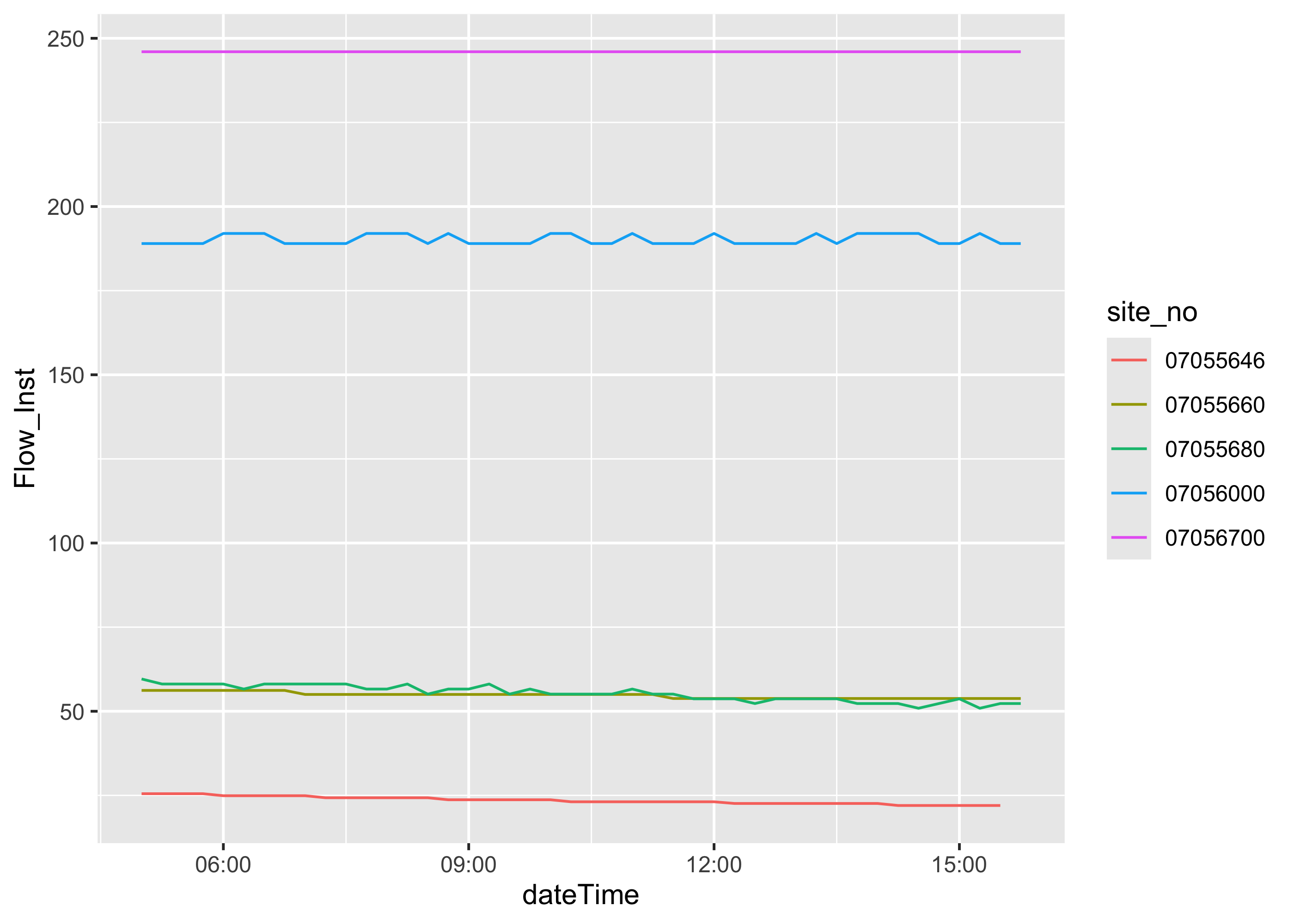
Now if we wanted to convert the data to hourly data saved at the end of the hour.

Create a new data frame so you can open both up and look back and forth to see what you are changing with each step

flowDat2 <- flowDat %>% 
  mutate(dateTime = as.POSIXct(dateTime, format = "%Y-%m-%d %H:%M:%S", tz = "UTC")) %>%
  mutate(date_hour = floor_date(dateTime, unit = "hour")) %>%
  group_by(site_no, date_hour) %>%  
  summarize(flow = mean(Flow_Inst)) %>% 
  ungroup()

# is there a relationship between flow and drainage area
ggplot(data = flowDat, aes(x = dateTime, y = Flow_Inst, color = site_no)) + 
     geom_line()+
     geom_line(data = flowDat2, aes(x = date_hour, y = flow , color = site_no),
               linetype="dashed")

We can also download daily data starting many years ago, including data starting in water year 2020 from these 5 sites on the Buffalo River.

flowDatdaily <- readNWISdv(whatSites$site_no, startDate = "2019-10-01", parameterCd = "00060", )
flowDatdaily <- renameNWISColumns(flowDatdaily)

We can plot the data using ggplot.

library(scales)

ggplot(data = flowDatdaily, aes(x = Date, y = Flow, color = site_no)) + 
     geom_line()+
     scale_y_continuous(breaks = seq(0, 500000, 5000) )+ 
     scale_x_date(breaks="6 month", labels=date_format("%Y-%m"),expand = c(0,0) )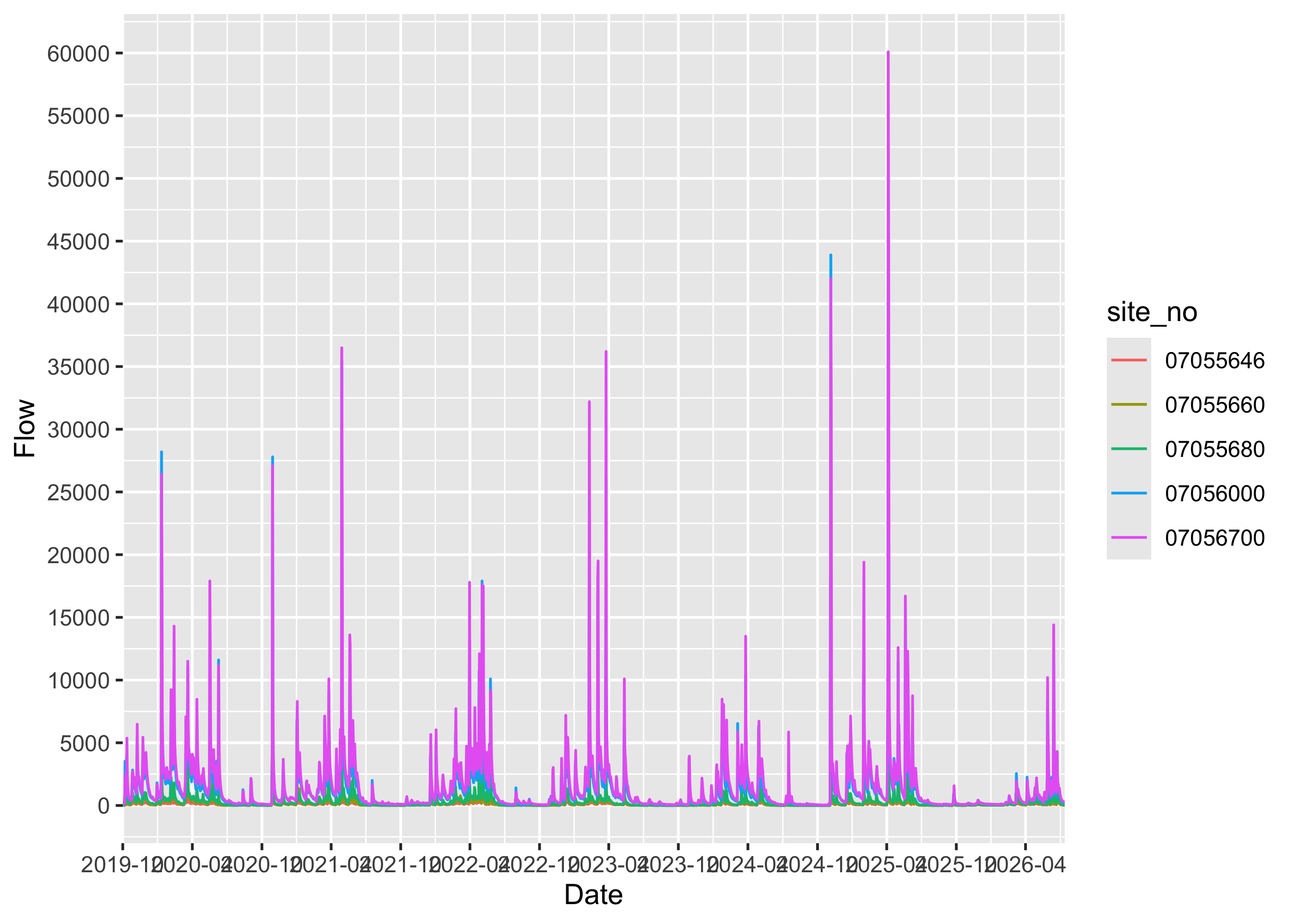

If you wanted to write out the gages instead of filtering the data, you can reference the site number directly in the function.

flowDatdailyone <- dataRetrieval::readNWISdv("07055646", startDate = "2019-10-01", parameterCd = "00060", statCd = "00003")

## Warning in dataRetrieval::readNWISdv("07055646", startDate = "2019-10-01", : NWIS servers are
## slated for decommission. Please begin to migrate to read_waterdata_daily.

## GET: https://waterservices.usgs.gov/nwis/dv/?site=07055646&format=waterml%2C1.1&ParameterCd=00060&StatCd=00003&startDT=2019-10-01

flowDatdailytwo <- readNWISdv(c("07055646", "07055660"), startDate = "2019-10-01", parameterCd = "00060")

## Warning in readNWISdv(c("07055646", "07055660"), startDate = "2019-10-01", : NWIS servers are
## slated for decommission. Please begin to migrate to read_waterdata_daily.

## GET: https://waterservices.usgs.gov/nwis/dv/?site=07055646%2C07055660&format=waterml%2C1.1&ParameterCd=00060&StatCd=00003&startDT=2019-10-01

25 Using R for data access

27 National Hydrography Dataset