23 National Hydrography Dataset
This module will teach you how to interact with the National Hydrography Dataset and river network data using the nhdplusTools package in R.
nhdplusTools along with data from the National Inventory of Dams.Author: Ed Stowe
Last update: 2026-03-23
Acknowledgements: Material was inspired by the nhdplusTools vignette developed by David Blodgett and Mike Johnson, the creators of the nhdplusTools package
23.1 Learning objectives
- Learn what the National Hydrography Dataset contains.
- Learn how to build and interact with watershed networks using the
nhdplusToolspackage inR. - Learn how R can facilitate analyses that bring together NHD data along with diverse datasets related to dams, stream gages, and land cover.
23.2 Background
The National Hydrography Dataset (NHD) is a database that represents the water drainage network of the U.S. It’s features include rivers, streams, lakes, canals and other waterbodies, as well as other features relevant to water management, such as stream gages and dams.
The NHD database is packed with information. Each stream segment, for example, is associated with over a hundred variables, including its length and Strahler stream order. Several attributes also relate a given segment to its neighboring segment, so that information about the entire watershed can be characterized.
NHD data can be downloaded from the web and accessed in GIS software but can be unwieldy. However, a useful package in R, the nhdplusTools package, makes it easy to perform a lot of common watershed related tasks, while harnessing other advantages of performing tasks in R, such as automating repetitive tasks.
In this module, we will investigate the watershed upstream of Juliette Dam, a former hydropower dam on the Ocmulgee River in Georgia. Discussions about removing the dam have been ongoing, and when this occurs, it can be helpful to consider habitat upstream that might be re-connected for migratory fishes.
For more information on the nhdplusTools package, visit the extensive package website.
23.3 Juliette Dam case study
To perform the main case study you need to load the nhdplusTools, as well as sf package for spatial operations and the tidyverse package for plotting and data wrangling. If you don’t have these packages installed, first uncomment the lines below and run the code to install them, before loading them.
Later in the module, we will also look at two applications that assess additional dams and land use upstream of Juliette Dam, and these applications will require two additional R packages as well.
23.3.1 Downloading NHD network data
# install.packages("nhdplusTools")
# install.packages("sf")
# install.packages("tidyverse")

library(tidyverse)
library(nhdplusTools)
library(sf)
To build our stream network upstream of Juliette Dam, we will first need its coordinates to find the nearest stream segment. With the coordinates, the below code creates a spatial point using the st_sfc function in the sf package. For this function, we need to tell it what the coordinates are (always listing longitude–the x coordinate–first). We also need to set the coordinate system (or crs). Here we give it 4269, which a code (called the EPSG) that is unique for each coordinate reference system. This one is a coordinate system for using latitude-longitude coordinates in North America.
Now we want to find an associated stream segment and catchment. Each stream segment is identified by an ID called a COMID. This ID also identifies a local catchment for that segment, which is the area that contributes surface flow to a given NHD segment. The COMID is also associated with numerous attributes that describe the stream segment and catchment.
We use the discover_nhdplus_id function to find the COMID and stream segment closest to our point.
Adding raindrop = true creates a downslope trace from our point location to nearest flowline, although that’s not very important in our case because our point is on the dam, in the middle of the river.
start_segment <- discover_nhdplus_id(start_point, raindrop = TRUE)

start_segment
## Simple feature collection with 2 features and 7 fields
## Geometry type: LINESTRING
## Dimension: XY
## Bounding box: xmin: -83.79481 ymin: 33.09087 xmax: -83.78007 ymax: 33.10659
## Geodetic CRS: WGS 84
## # A tibble: 2 × 8
## id gnis_name comid reachcode raindrop_pathDist measure intersection_point
## <chr> <chr> <int> <chr> <dbl> <dbl> <list>
## 1 nhdFlowline Ocmulgee River 6336752 03070103000084 26.2 97.7 <dbl [2]>
## 2 raindropPath <NA> NA <NA> NA NA <dbl [0]>
## # ℹ 1 more variable: geometry <LINESTRING [°]>
start_comid <- as.integer(start_segment$comid)[1]

start_comid
## [1] 6336752This returns a spatial dataframe with two rows, one for our stream segment of interest containing the important COMID, and one that is the path of our raindrop.
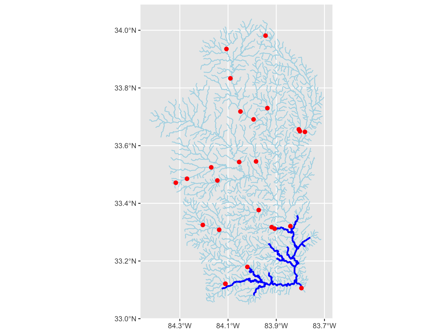
Now we visualize the starting point and stream segment in ggplot. The geom_sf function in ggplot conveniently plots spatial objects created with the sf package. We adjust the x-axis labels to make them more legible.
ggplot()+
  geom_sf(data = start_segment)+
  geom_sf(data = start_point, color = "red", size = 4)+
  scale_x_continuous(breaks = seq(-83.794, -83.782, .004))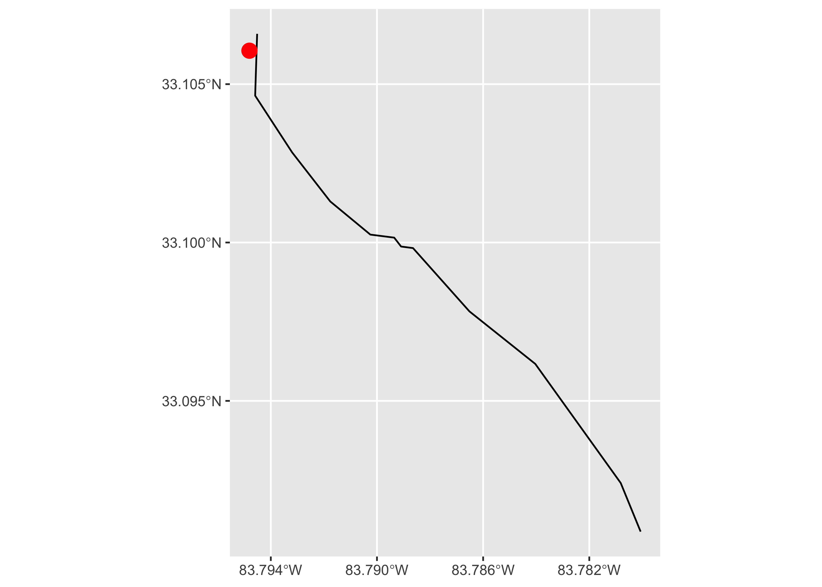
We now build the river network upstream of our point using the Network Linked Data Index which spatially links several different hydrological data sources, including USGS stream gages. To do that, we first create a list object, in which we indicate that we are using COMID data (featureSource = "comid"), and then the value of the COMID which we stored earlier in the start_comid object. Then, we use the navigate_nldi function, and set it to look for upstream tributaries by setting mode = "UT. Other options include upstream mainstem (UM) and downstream mainstem and diversions (DM and DD, respectively). We indicate to stop navigating after 1,000 km.
nldi_feature <- list(featureSource = "comid",
                     featureID = start_comid)

flowline_nldi <- navigate_nldi(nldi_feature, mode = "UT",
                               distance_km = 1000)
The data returned with navigate_nldi is a list object with two spatial dataframes, one for our origin segment, and one of the upstream stream network.
We can plot our network in ggplot. We plot the original segment and the new steam network by referring to the different list elements using the $ symbol.
ggplot()+
  geom_sf(data = flowline_nldi$UT, linewidth = 0.5, color = "lightblue")+
  geom_sf(data = flowline_nldi$origin, linewidth = 1, color = "black")+
  geom_sf(data = start_point, size = 1, linewidth = 2, color = "red") +
  scale_x_continuous(breaks = seq(-84.4, -83.8, .2))
It’s great to get an upstream river network so easily, but downloading the flowline with the NLDI function only provides the geometry and COMID for flowlines. What if you want more of the data from the very extensive NHD dataset?
To do that we can download a subset of the NHD layer with the subset_nhdplus function, which will get us all of the attributes associated with our stream segments, as well as other NHD layers.
The subset_nhdplus function has several options. See comments in the code for a brief explanation, or the function description here for more info.
nhd_sub <-subset_nhdplus(comids = as.integer(flowline_nldi$UT$nhdplus_comid),
                         nhdplus_data = "download", # Or use nhdplus_path()
                         flowline_only = FALSE,     # FALSE downloads flowlines, catchments, waterbodies, etc.
                         return_data = TRUE)        # FALSE downloads to file; TRUE downloads into list in R session


names(nhd_sub)
## [1] "NHDFlowline_Network" "CatchmentSP" "NHDArea"
## [4] "NHDWaterbody" "NHDFlowline_NonNetwork"The data returned with subset_nhdplus is again a list object with spatial dataframes, in this case the five different ones listed above, including flowlines, but also with other useful data such as the catchment layer.
Here we create standalone layers from the nhd_sub object.
flowline <- nhd_sub$NHDFlowline_Network
catchment <- nhd_sub$CatchmentSP
waterbody <- nhd_sub$NHDWaterbody
Now that we have more info for each segment, we can do a lot more. For example, we can plot just bigger streams within the network (i.e., streams with a Strahler stream order of 3 or above).
bigger_streams <- filter(flowline, streamorde > 2)

ggplot()+
  geom_sf(data = flowline, linewidth = 1, color = "blue")+
  geom_sf(data = bigger_streams, linewidth = 1.5, color = "grey30")  +
  scale_x_continuous(breaks = seq(-84.4, -83.8, .2))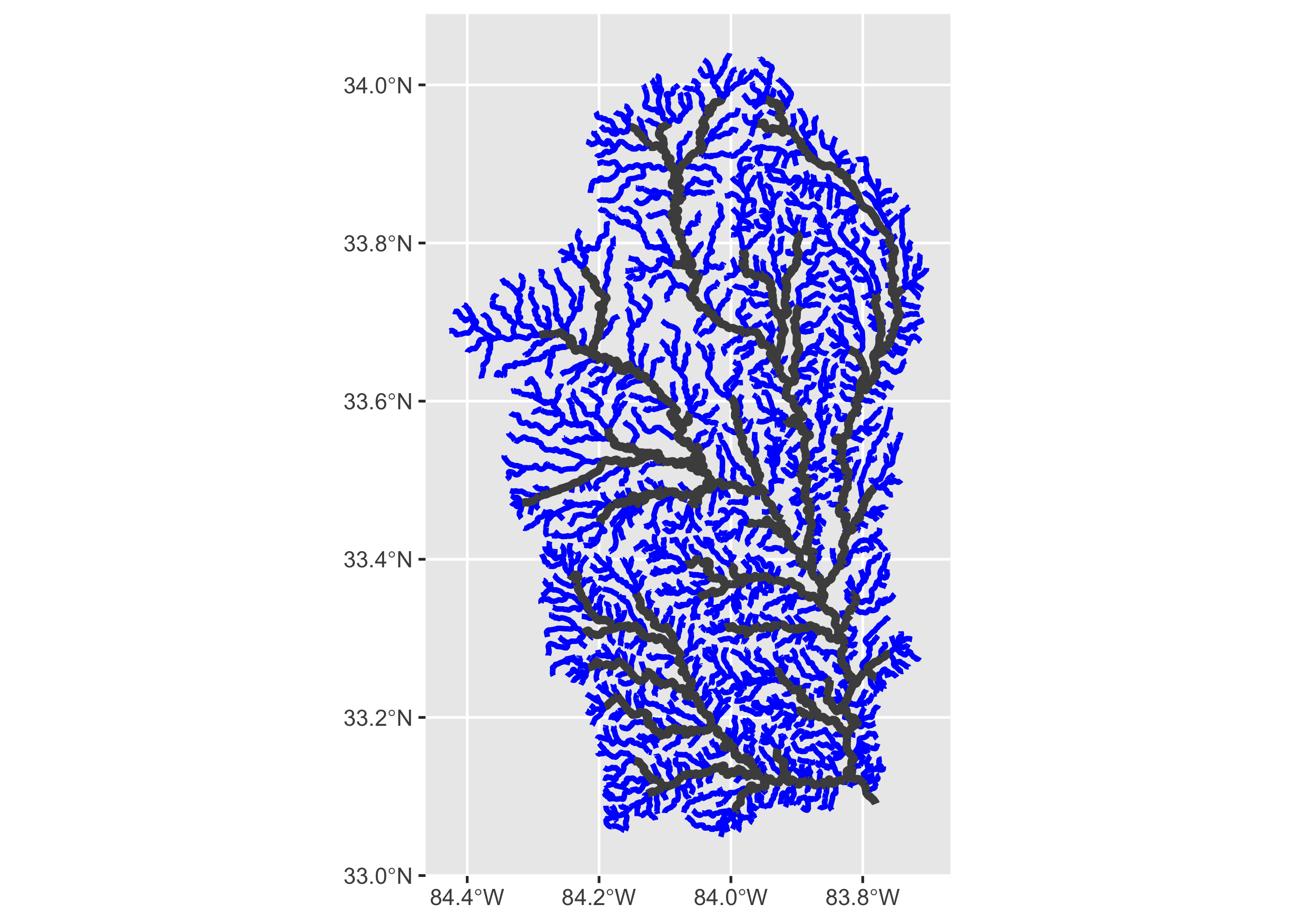
We can also calculate the length of flows upstream of the dam in kilometers:
total_upstream_km <- sum(flowline$lengthkm)With the full flowline data, each segment has a ton of attributes that are useful. We print all of those attributes below. More information on these attributes can be found online, including here.
names(flowline)## [1] "comid" "fdate" "resolution" "gnis_id" "gnis_name" "lengthkm"
## [7] "reachcode" "flowdir" "wbareacomi" "ftype" "fcode" "shape_length"
## [13] "streamleve" "streamorde" "streamcalc" "fromnode" "tonode" "hydroseq"
## [19] "levelpathi" "pathlength" "terminalpa" "arbolatesu" "divergence" "startflag"
## [25] "terminalfl" "dnlevel" "uplevelpat" "uphydroseq" "dnlevelpat" "dnminorhyd"
## [31] "dndraincou" "dnhydroseq" "frommeas" "tomeas" "rtndiv" "vpuin"
## [37] "vpuout" "areasqkm" "totdasqkm" "divdasqkm" "tidal" "totma"
## [43] "wbareatype" "pathtimema" "hwnodesqkm" "maxelevraw" "minelevraw" "maxelevsmo"
## [49] "minelevsmo" "slope" "elevfixed" "hwtype" "slopelenkm" "qa_ma"
## [55] "va_ma" "qc_ma" "vc_ma" "qe_ma" "ve_ma" "qa_01"
## [61] "va_01" "qc_01" "vc_01" "qe_01" "ve_01" "qa_02"
## [67] "va_02" "qc_02" "vc_02" "qe_02" "ve_02" "qa_03"
## [73] "va_03" "qc_03" "vc_03" "qe_03" "ve_03" "qa_04"
## [79] "va_04" "qc_04" "vc_04" "qe_04" "ve_04" "qa_05"
## [85] "va_05" "qc_05" "vc_05" "qe_05" "ve_05" "qa_06"
## [91] "va_06" "qc_06" "vc_06" "qe_06" "ve_06" "qa_07"
## [97] "va_07" "qc_07" "vc_07" "qe_07"
## [ reached getOption("max.print") -- omitted 38 entries ]If we wanted to understand upstream affects of removing a dam and increasing connectivity for fish, there are several things we might want to figure out, including whether the upstream land use is likely to support fish, and how much riverine habitat will actually be connected by removing a dam. The following code will use data from other packages along with our river network to provide a window into those questions.
23.3.2 Use EPA StreamCat data for land use
The EPA has created a StreamCat dataset which contains substantial information about each catchment found in the NHD layer. We’re going to use that dataset to look a little bit at land use in our upstream watershed.
This dataset can be downloaded online, but we’ll use the StreamCatTools package to pull landuse data directly into R. This package is not hosted on CRAN because it’s still being developed. So, users will need to “uncomment” the following code and run it to download StreamCatTools the first time they do this analysis.
#install.packages("remotes")
#library(remotes)
#install_github("USEPA/StreamCatTools", build_vignettes=FALSE)
Once it’s downloaded, we can load the StreamCatTools package. There are several ways to download NLCD data with this package (see more here), but an easy way to do this is to use the sc_nlcd function. Here, we indicate that we are interested in catchment data (cat), as opposed to watershed data (ws) which is at a bigger scale, and then we are interested in data from Georgia, in the latest year for which NLCD data is available, which is 2019.
library(StreamCatTools)

ga_nlcd <- sc_nlcd(aoi = 'cat', state='GA', year = '2019')

names(ga_nlcd)
We can see that in addition to a column for the catchment COMID, we have the percentage of various land cover types, such as percentage mixed forest (pctmxfst2019cat) and columns for urban land cover (high, medium, low, and open).
We’re only interested in land cover data for our watershed, not all of GA. So, we use left_join to merge the land cover data with the catchment layer. This join is done by matching COMIDs, although the column with COMIDs is called featureid in the catchment dataset.
If we are interested in, say, urban land cover, we can sum across the different categories of urban land cover data, which is accomplished by summing across all columns with names that match the string “urb”.
catchment_lc <- left_join(catchment, ga_nlcd,
                    by = c("featureid" = "comid")) %>%
  mutate(pct_urb = rowSums(across(matches("urb"))))
Let’s plot our catchments now to see how urban the different catchments are above the dam.
ggplot()+
  geom_sf(data = catchment_lc, aes(fill = pct_urb))+
  geom_sf(data = filter(flowline, streamorde > 2),
     linewidth = 1.5, color = "blue")+
  scale_fill_continuous(type = "viridis")+
  scale_x_continuous(breaks = seq(-84.4, -83.8, .2))
Based on this, the headwaters of this basin have a lot of urban land cover, approaching 100% in some cases, with clear ramifications for the kinds of organisms that might persist there.
23.3.3 Use NID for dams
Another consideration for thinking about connectivity in the watershed upstream of Juliette concerns how the stream network is impacted by dams.
To take a look at this, we’ll use data from the National Inventory of Dams (NID), which is a database managed by USACE that documents all known dams in the U.S.
The NID can be queried and downloaded online, but we can also use the dams package in R to download a subset of the dams.
Here we load the dams package. (Install the package the first time you use it.) We can quickly filter our NID to just Georgia so that it’s more wieldy.
#install.packages("dams")
library(dams)

# Download subset of dam data
nid <- dams::nid_subset %>%
  filter(state == "GA")
Next, we can make the NID a spatial object with the st_as_sf function in the sf package. Again, we need to tell the function which columns contain the x- and y-coordinates of each dam, as well as the coordinate system.
# Make NID data a spatial object; set coordinate reference system (crs) to Lat Long EPSG
nid_sf <- st_as_sf(nid, coords = c("longitude", "latitude"), crs = 4269)

names(nid_sf)
## [1] "recordid" "dam_name" "nidid" "county"
## [5] "owner_type" "dam_type" "purposes" "year_completed"
## [9] "nid_height" "max_storage" "normal_storage" "nid_storage"
## [13] "hazard" "eap" "inspection_frequency" "state_reg_dam"
## [17] "spillway_width" "volume" "number_of_locks" "length_of_locks"
## [21] "width_of_locks" "source_agency" "state" "submit_date"
## [25] "party" "numseparatestructures" "permittingauthority" "inspectionauthority"
## [29] "enforcementauthority" "jurisdictionaldam" "geometry"We need to find which stream segments are associated with each dam so we can see where the river network has obstructions. But, our flowline object is a line feature, which can’t be intersected/overlaid directly by a point object (our dam object), because even if the point and line were extremely close in space, they would not overlap. Therefore, to see where our flowlines and dam points meet, we’ll turn the line object into a polygon which can then be intersected with our dam points. We’ll do this using the st_buffer function.
First, we’ll imagine that we’re interested in habitat for a fish that only likes larger streams, so we’ll filter theflowline dataframe to just stream orders greater than 2. We may want to buffer our line by about 100 meters or so. However, to do this, we first need to re-project the coordinate system to one that uses the metric system instead of latitude and longitude (here, NAD83, Zone 17 N, which has an EPSG of 26917). At the end of each line, we also want the buffer to be completely flat so that each segment will be flush with the next one, as opposed to having rounded ends that overlap (hence the code endCapStyle = "Flat").
# Create buffered streams of third order and bigger streams
# Transform to NAD83 zone 17n so can use meters for buffer
stream100 <- filter(flowline, streamorde > 2) %>%
  st_transform(crs = 26917) %>%
  st_buffer(dist = 100, endCapStyle="FLAT")
Now we can use the st_intersection function to see which dams intersect with the larger streams in our network. Note: to do this, we also need to convert the coordinate system of our dams to be the same as our buffered stream segments.
The second code below simply shows that each dam is now associated with a COMID, and thus a specific stream segment.
#Dams that intersect with mainstem buffer
nid100 <- nid_sf %>%
  st_transform(crs = 26917) %>%
  st_intersection(stream100)
## Warning: attribute variables are assumed to be spatially constant throughout all geometries## Simple feature collection with 6 features and 2 fields
## Geometry type: POINT
## Dimension: XY
## Bounding box: xmin: 222446 ymin: 3715728 xmax: 240149.9 ymax: 3764001
## Projected CRS: NAD83 / UTM zone 17N
## # A tibble: 6 × 3
## dam_name comid geometry
## <chr> <int> <POINT [m]>
## 1 ATLANTA AUTOMOTIVE DISTRIBUTION CENTER DETENTION DAM 6330502 (227982.4 3764001)
## 2 JACK TURNER RESERVOIR DAM 6330976 (227895.6 3736098)
## 3 MILSTEAD 6331062 (222446 3731921)
## 4 CORNISH CREEK RESERVOIR DAM 6331166 (240149.9 3726872)
## 5 TWIN HILLS LAKE 6331166 (239756.8 3727592)
## 6 CAPES SAUSAGE COMPANY LAKE DAM 6331416 (222935.6 3715728)Now we can see how bifurcated our larger stream network is. To do this, we simply filter our original flowline so to remove all small streams and all streams with COMIDs that are found associated with dams (i.e., COMID values that are now found in the nid100 object and thus segments with a dam).
# Filter flowline to just
flow_no_dam <- filter(flowline,
                      streamorde > 2,
                      !comid %in% nid100$comid)

plot(flow_no_dam$geometry)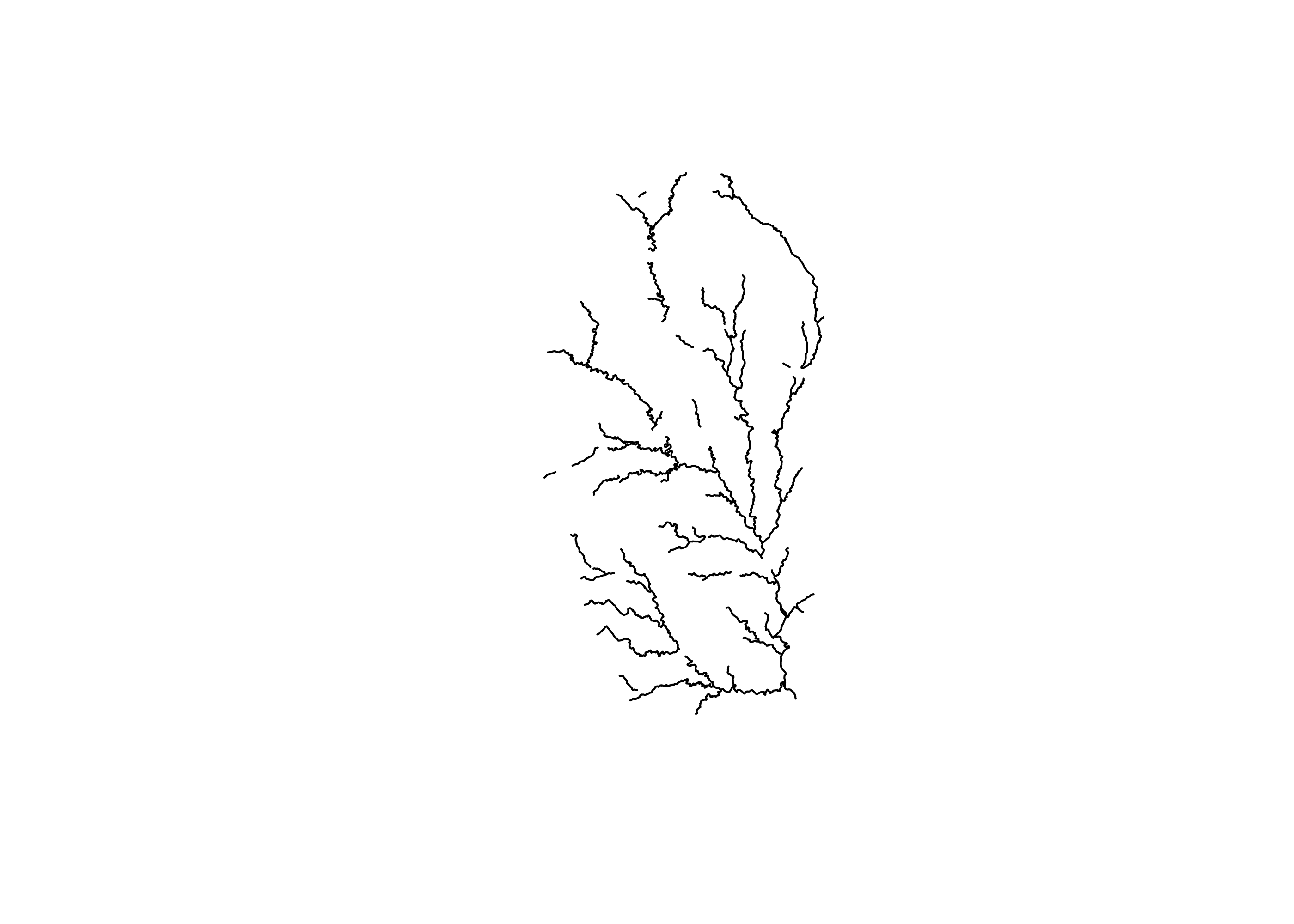
Based on this plot, we can now see that the upstream network is definitely bisected by dams.
What if we want to find out how much mainstem river would be opened up by removing this dam?
We can use some of the network attributes in our streamlayer to answer this question, in particular the fromnode and tonode attributes. The fromnode is a unique code representing the upstream end of a stream segment, and it has the identical value as the tonode of the downstream end of the segment immediately upstream of it. So, we can use the values of these two nodes to map the upstream watershed of our disjointed network, and the navigation will stop when we get to dams or small streams.
First, we can use the COMID of our downstream-most segment to find the value of the fromnode that we want to start with.
What is that COMID? It’s stored in this object that we created at the outset:
start_comid## [1] 6336752We can use the fromnode in this segment to find adjacent stream segments
from_node <- flowline$fromnode[flowline$comid == start_comid]

from_node
## [1] 270015756To show how this works, here we show that if we filter our flowline to just flowline where the tonode equals the initial fromnode, we get a new steam segment:
## Simple feature collection with 1 feature and 137 fields
## Geometry type: LINESTRING
## Dimension:     XY
## Bounding box:  xmin: -83.79718 ymin: 33.10659 xmax: -83.79452 ymax: 33.11509
## Geodetic CRS:  NAD83
## # A tibble: 1 × 138
##     comid fdate               resolution gnis_id gnis_name     lengthkm reachcode flowdir wbareacomi
## *   <int> <dttm>              <chr>      <chr>   <chr>            <dbl> <chr>     <chr>        <int>
## 1 6336742 2008-12-10 00:00:00 Medium     356443  Ocmulgee Riv…    0.995 03070103… With D…  120049944
## # ℹ 129 more variables: ftype <chr>, fcode <int>, shape_length <dbl>, streamleve <int>,
## #   streamorde <int>, streamcalc <int>, fromnode <dbl>, tonode <dbl>, hydroseq <dbl>,
## #   levelpathi <dbl>, pathlength <dbl>, terminalpa <dbl>, arbolatesu <dbl>, divergence <int>,
## #   startflag <int>, terminalfl <int>, dnlevel <int>, uplevelpat <dbl>, uphydroseq <dbl>,
## #   dnlevelpat <dbl>, dnminorhyd <dbl>, dndraincou <int>, dnhydroseq <dbl>, frommeas <dbl>,
## #   tomeas <dbl>, rtndiv <int>, vpuin <int>, vpuout <int>, areasqkm <dbl>, totdasqkm <dbl>,
## #   divdasqkm <dbl>, tidal <int>, totma <dbl>, wbareatype <chr>, pathtimema <dbl>, …
Given that proof of concept, we just need to package this in a for-loop, seen below, so that we can iterate through all the pairs of to and from nodes. In this example, we simply create an empty vector to store all of the COMIDs that are encountered. And in each iteration of the loop, we use the fromnode values of the new segments to look for the tonode values of the next set of segments.
# Empty vector to store new comids
segs_all <- vector()

for (i in 1:length(flow_no_dam)){

  to_segs <- filter(flow_no_dam, tonode %in% from_node)
  from_node <- unique(to_segs$fromnode)

  segs_all <- c(segs_all, to_segs$comid)

if(nrow(to_segs) == 0) {break}
  }
Once we have the COMIDs of our newly navigated area, we can filter the original flowline just to the newly-opened mainstem sterams.
Finally, let’s plot the new network of larger streams that would be connected if the dam in question were removed, along with dams found on the river network in general, and the total upstream watershed.
ggplot()+
  geom_sf(data = flowline, color = "lightblue", linewidth = .5)+
  geom_sf(data = new_flow, color = "blue", linewidth = 1)+
  geom_sf(data = nid100, color = "red", size = 2)+
  scale_x_continuous(breaks = seq(-84.5, -83.5, .2 ))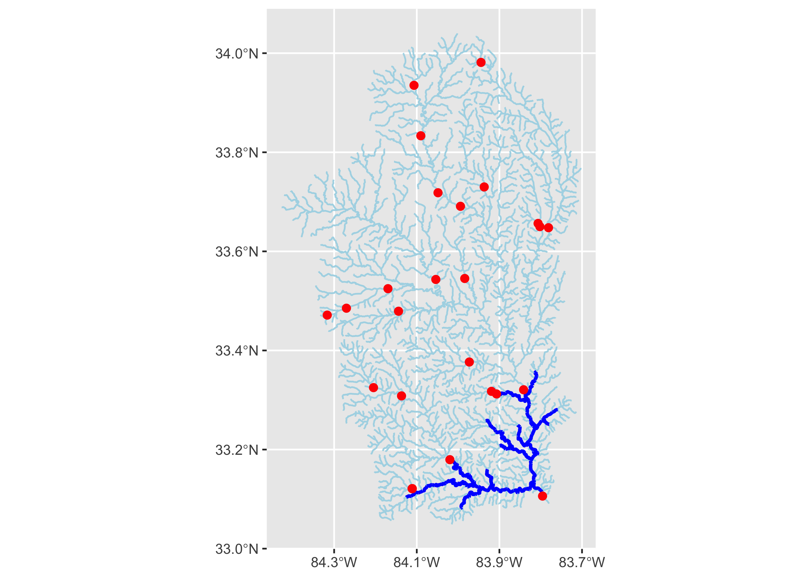
There’s a lot we could do with this new network, but let’s just compare the its length to the length of the overall network.
total_upstream_km## [1] 3926.602
sum(new_flow$lengthkm)## [1] 159.549
sum(new_flow$lengthkm)/total_upstream_km## [1] 0.04063284This suggests that removing Juliette Dam would open up approximately 159 kms of upstream mainstem habitat. Of course, it’s likely a bit more, as this does not conisder partial portion of the stream segments that contain dams, but this amounts should be fairly trivial, as stream segments in our network are on average 1.37.
23.3.4 Finding streamgages
The applications for the nhdplusTools package are extensive. One final application we highlight is to find gages upstream of a point that might be used for a hydrologic analysis. The code below, highly analogous to the code that we have already used, finds gages and flow networks upstream of a gage of interest, in this case a gage in Madison, WI.
# Create starting nldi feature
nldi_feature <- list(featureSource = "nwissite",
                     featureID = "USGS-05428500")

# Create a flowline from this feature to extract COMIDs
flowline_nldi <- navigate_nldi(nldi_feature,
                               mode = "upstreamTributaries",
                               distance_km = 1000)

# Download full NHD flow data from these COMIDs
gage_download <-subset_nhdplus(comids = as.integer(flowline_nldi$UT$nhdplus_comid),
                                  nhdplus_data = "download",
                                  return_data = TRUE)

# Extract flow network from the download
flowline_nwis <- gage_download$NHDFlowline_Network

# Find all of the upstream gages
upstream_nwis <- navigate_nldi(nldi_feature,
                               mode = "upstreamTributaries",
                               data_source = "nwissite",
                               distance_km = 1000)

# Plot gages and stream network
ggplot()+
  geom_sf(data = flowline_nwis, linewidth = 1, color = "blue")+
  geom_sf(data = upstream_nwis$UT_nwissite,
     size = 1.5, linewidth = 2, color = "red")
23.4 Summary
- The National Hydrography Data has a huge amount of information that is fundamental to water resource management, but can be unwieldy to use
- The
nhdplusToolspackage makes using NHD data simple and powerful - Performing this analysis in
Rmakes it simple to access data from other packages as well as use powerfulRprogramming tool while interacting with NHD data