13 Random Forest
This module will teach you how to run a full machine learning workflow with a random forest model using the tidymodels package in R.
Authors: Ed Stowe (writing, editing)
Last update: 2026-03-03
Acknowledgements: Case study includes code that was adapted from demonstration analyses by Julia Silge on random forest and partial dependence plots, used under Creative Commons Attribution-ShareAlike 4.0 International License
13.1 Learning objectives
- Understand how random forest models works and when they are useful
- Carry out a full machine learning workflow
- Learn how to tune and assess a random forest model and determine which variables are important
13.2 Background
13.2.1 What is machine learning?
Machine learning constitutes using algorithms that can learn to recognize patterns in data and then make predictions in new scenarios.
13.2.2 When is it most useful?
In general, ML is most useful when prediction are more important than explanation; and when there is an adequate amount of data. ML models work better with more data, typically when there are at least a few hundred observations.
13.2.3 Can I do machine learning
Yes. Machine learning (ML) has a reputation for complexity and technical difficulty. But many machine learning algorithms are relatively simple, have been in use for decades, and are now fairly accessible via R packages like the tidymodels
13.2.4 What programs can I use for ML?
There are lots of tools/programs for running ML algorithms, but one very accessible way is to use the tidymodels packages in R, which provides an integrated framework for using dozens of different ML algorithms. Different algorithms might make sense for different applications. Here we use random forest, an algorithm that’s been popular for decades because of its flexibility, performance, relative ease, and suitability for tabular data (i.e., spreadsheets).
13.2.5 How does random forest work
Random forest is an extension of a technique called decision trees. Decision trees, like other supervised machine learning algorithms, are designed to predict outcomes based on input data. There are two main types of outcomes that decision trees might predict: - Classification: predicting categorical outcomes (e.g., present/absent; male/female, etc.) - Regression: predicting numeric outcomes (e.g., abundance of fish; number of species, etc.)
Input data is used to identify break points, called decision nodes, in the data that help predict what the outcome might be. For example, if we were to predict whether a given passenger survived the sinking of the Titanic, the first decision node (i.e., the most informative) would be whether the person was male or female. Other input variables, like the age of the passenger, would likely make up other important nodes in the tree, and the final prediction (i.e., did the person survive or note?) is denoted by the leaf node.
Decision trees are versatile and interpretable, but they often learn the data that they are trained on too well, which is called being “overfit.” Overfitted models tend to do poorly when used in prediction, because they are not general enough.
Random forest (and some similar algorithms) help overcome the problem of overfitting by leveraging the predictions of many distinct trees. It does this by:
- Creating many different decision trees, each using a random subset of the data (called bagging).
- Building each tree using only a few randomly chosen predictor variables.
- Generating independent predictions from each tree.
- Combining the predictions of the different trees by selecting the prediction that the most trees agree on.
Using random data and input variables for each tree has been shown to increase the overall accuracy and generalizability of these models compared to single decision trees.
13.3 Case study
Here we present a case study using machine learning to predict whether or not bluegill will be present at different sites in the Upper Mississippi River based on habitat covariates. Bluegill are often the focus of restoration efforts there, so better understanding what controls bluegill presence can help determine what features restoration should focus on. This analysis includes steps that are fundamental to all machine learning workflows and also relevant in many other models forms as well, which include:
- Splitting the data: partitioning data so that models can be trained and then tested on independent data
- Tuning and training models: using the training processing to examine model fit and determine which model specifications (i.e., hyperparameters) yield the best predictions
- Assessing model performance
- Predicting independent data: compare model predictions to test dataset to see if it performs well
13.3.1 Add packages
This case study will use the tidymodels package. We will also load the following packages:
- tidyverse for plotting and data-handling
- doParallel for tuning models in parallel
- vip for calculating variable importance
- partial for making partial dependence plots
These packages should be installed if you have not used them before (e.g., install.packages("vip"))
## Warning: package 'pdp' was built under R version 4.4.3First, we can import the bluegill occupancy dataset, and look at the data structure ### Import dataset
blgl <- read_csv("data/bluegill.csv")## Rows: 1422 Columns: 11
## ── Column specification ───────────────────────────────────────────────────────────────────────────────────
## Delimiter: ","
## chr (1): pool
## dbl (10): occ, utm_e, utm_n, period, secchi, temp, depth, cond, current, do
##
## ℹ Use `spec()` to retrieve the full column specification for this data.
## ℹ Specify the column types or set `show_col_types = FALSE` to quiet this message.
str(blgl)## spc_tbl_ [1,422 × 11] (S3: spec_tbl_df/tbl_df/tbl/data.frame)
## $ occ : num [1:1422] 0 1 1 1 0 1 1 0 0 0 ...
## $ utm_e : num [1:1422] 734608 734108 734608 735008 734108 ...
## $ utm_n : num [1:1422] 4648501 4648551 4648501 4650751 4648601 ...
## $ pool : chr [1:1422] "13" "13" "13" "13" ...
## $ period : num [1:1422] 2 3 3 2 2 3 3 1 1 1 ...
## $ secchi : num [1:1422] 35 60 48 46 NA 29 42 42 32 NA ...
## $ temp : num [1:1422] 22.7 20.7 16.6 23.8 NA 18.9 15.8 27.8 25.4 NA ...
## $ depth : num [1:1422] 0.5 0.6 0.9 1.2 NA 0.9 1 0.8 0.8 NA ...
## $ cond : num [1:1422] 404 464 321 376 NA 459 312 367 492 NA ...
## $ current: num [1:1422] 0 0 0 0.08 NA 0.06 0.06 0 0 NA ...
## $ do : num [1:1422] 11.8 4.4 10.5 8 NA 7.4 9.9 8.2 5.3 NA ...
## - attr(*, "spec")=
## .. cols(
## .. occ = col_double(),
## .. utm_e = col_double(),
## .. utm_n = col_double(),
## .. pool = col_character(),
## .. period = col_double(),
## .. secchi = col_double(),
## .. temp = col_double(),
## .. depth = col_double(),
## .. cond = col_double(),
## .. current = col_double(),
## .. do = col_double()
## .. )
## - attr(*, "problems")=<externalptr>We see that all but one of these variables are numeric. However, for our classification algorithm, we need to convert the presence/absence column (occ for occupancy) to a factor. We also have two other categorical variables that should be factors: pool for the number of the navigation pool, and period, for the season (with 2, 3, 4 being approximately spring, summer, and fall, respectively).
We may also want to explore the data a bit. Here we look to see if there are any patterns of bluegill occupancy across space, and based on depth.
filter(blgl, depth < 4) %>%
ggplot()+
geom_point(aes(utm_e, utm_n, color = depth, shape = occ))+
  facet_wrap(~pool, scales = "free")+
  scale_color_viridis_c()+
  theme_void() +
  labs(shape = "Presence",
       color = "Depth (m)")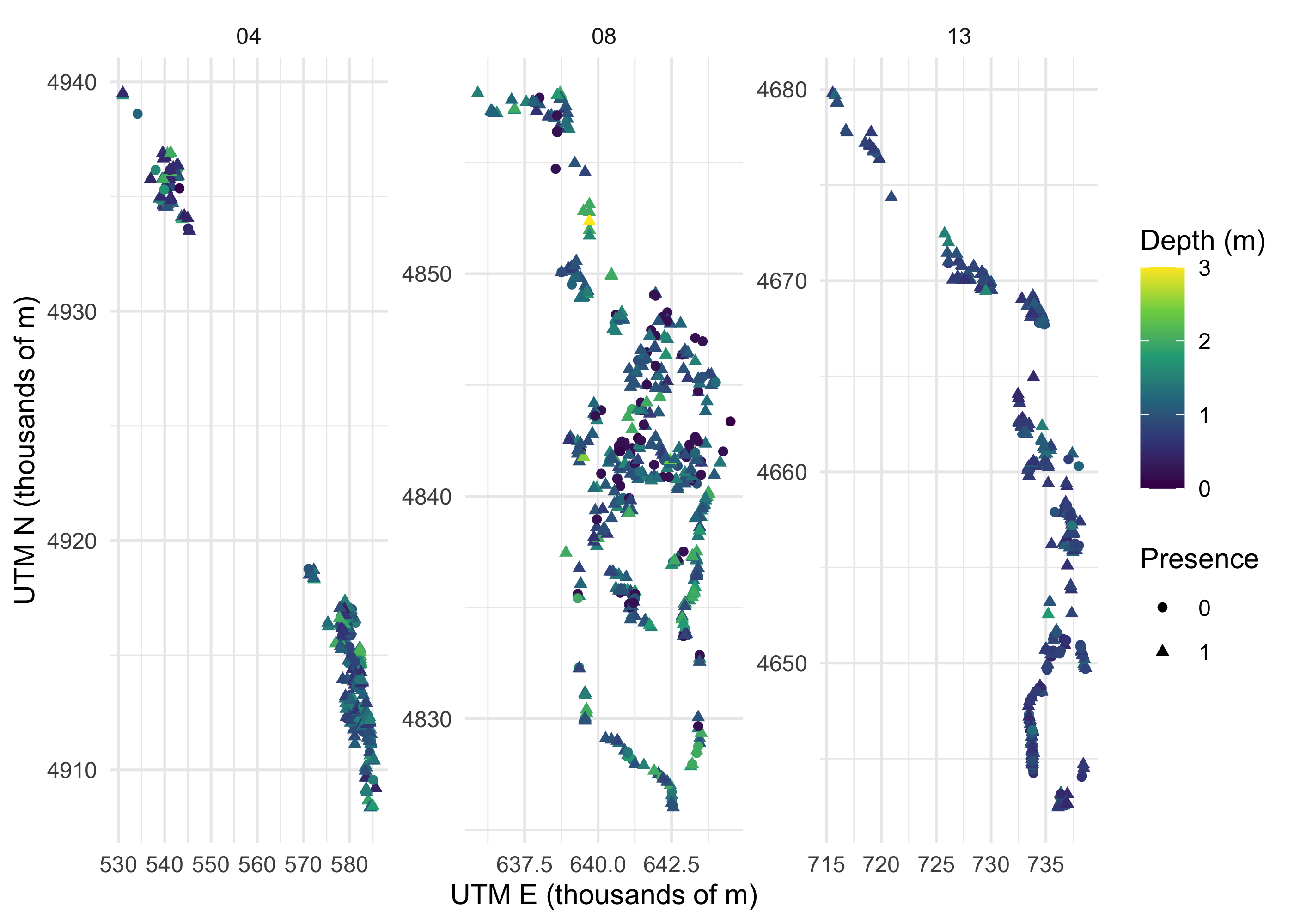
Clearly these data are complex, and modeling should help us make sense of it.
13.3.2 Data partitioning
Splitting the data is very important so that we have some independent data on which to judge our models performance. Here we split 75% of the data into the dataset that will be used to train the model, and the remainder into the dataset for testing/assessing our model. 75% is the tidymodels default splitting proportion.
blgl_split <- initial_split(blgl, strata = occ, prop = .75)
blgl_train <- training(blgl_split)
blgl_test <- testing(blgl_split)
13.3.3 Pre-processing with recipes
Build a recipe for data preprocessing.
First, we must tell the recipe() what our model is going to be (using a formula here) and what our training data is. The recipe is where we can do lots of helpful data manipulations, such as normalizing the data (step_normalize()), replacing categorical variables with dummy variables (step_dummy), adding interactions (step_interact()), and numerous other options. Random forest models needed fewer data transformations than many algorithms, so we’ll just to one powerful transformation: step_impute_bag(). This uses a machine learning algorithm to impute missing variables, since we can’t have any missing predictor data to run this or many other machine learning algorithm. Another option would be to remove any rows with missing data (using step_naomit()), but that would remove a lot of data.
blgl_rec <- recipe(occ ~ ., data = blgl_train) %>%
  step_impute_bag(all_predictors())
ALthough not strictly necessary, to see what the data look like after applying transformations, we can use the functions prep and then juice. The juiced dataframe now shows us what our data will look like when it’s fed into the ML algorithm.
blgl_prep <- prep(blgl_rec)
juiced <- juice(blgl_prep)
13.3.4 Model specifications with parsnip
We will specify our random forest model. This is where we tell the model whether to try any different combinations of the hyperparameters (i.e., whether to tune the model). In this case, we’re going to set the number of trees in our model to be 1,000, but we will tune 2 other hyperparameters. The mtry parameter controls how many variables we’ll include in each model, and the min_n hyperparameter controls tree complexity: it indicates the minimum number of data points needed in a node for that node to be split, so higher values of min_n will force trees to be less complex. Tuning both of these parameters will help us find a more predictive model. For the model specification, we also indicate that we want to run our random forest using the version of the algorithm as implemented by the ranger package, and we want to do classification as opposed to regression.
13.3.5 Workflow
Next we set up our workflow. This is simply where we indicate what recipe and model we will use.
13.3.6 Tune hyperparameters
Now we’re ready to tune the hyperparameters. We need to create a set of cross-validation resamples to use for tuning. This means we’ll divide our training data into 10 slices, and sequentially fit models with different hyperparameters using 9 of the slices, and testing it on the 10th slice. This is how we’ll figure out the best hyperparameters.
blgl_folds <- vfold_cv(blgl_train, v = 10)We will use the tune_grid function to tune our model across a grid of hyperparameters (using grid = 20 will automatically pick 20 grid points automatically, but these can also be chosen by the user).
We will use parallel processing to make this go faster, but note that this could take about 1-2 minutes, depending on your computer.
doParallel::registerDoParallel()

tune_mod <- tune_grid(
  tune_wf,
  resamples = blgl_folds,
  grid = 20
)

tune_mod
## # Tuning results
## # 10-fold cross-validation
## # A tibble: 10 × 4
## splits id .metrics .notes
## <list> <chr> <list> <list>
## 1 <split [959/107]> Fold01 <tibble [60 × 6]> <tibble [0 × 3]>
## 2 <split [959/107]> Fold02 <tibble [60 × 6]> <tibble [0 × 3]>
## 3 <split [959/107]> Fold03 <tibble [60 × 6]> <tibble [0 × 3]>
## 4 <split [959/107]> Fold04 <tibble [60 × 6]> <tibble [0 × 3]>
## 5 <split [959/107]> Fold05 <tibble [60 × 6]> <tibble [0 × 3]>
## 6 <split [959/107]> Fold06 <tibble [60 × 6]> <tibble [0 × 3]>
## 7 <split [960/106]> Fold07 <tibble [60 × 6]> <tibble [0 × 3]>
## 8 <split [960/106]> Fold08 <tibble [60 × 6]> <tibble [0 × 3]>
## 9 <split [960/106]> Fold09 <tibble [60 × 6]> <tibble [0 × 3]>
## 10 <split [960/106]> Fold10 <tibble [60 × 6]> <tibble [0 × 3]>We can plot the accuracy of our models (using area under the curve, or “AUC”) to see which values of our hyperparameters are best. AUC is a score that indicates the balance between the sensitivity and specificity of a model, and thus is a good measure of model generalizability.
It appears that min_n values below ~8 and mtry values between 4 and 7 are best.
tuning_results <- collect_metrics(tune_mod)

# Subset to just ROC AUC results for plotting
results_auc <- tuning_results %>%
  filter(.metric == "roc_auc")

results_auc %>%
  dplyr::select(mean, min_n, mtry) %>%
  pivot_longer(min_n:mtry,
    values_to = "value",
    names_to = "parameter"
  ) %>%
  ggplot(aes(value, mean, color = parameter)) +
  geom_point(show.legend = FALSE) +
  facet_wrap(~parameter, scales = "free_x") +
  labs(x = NULL, y = "AUC")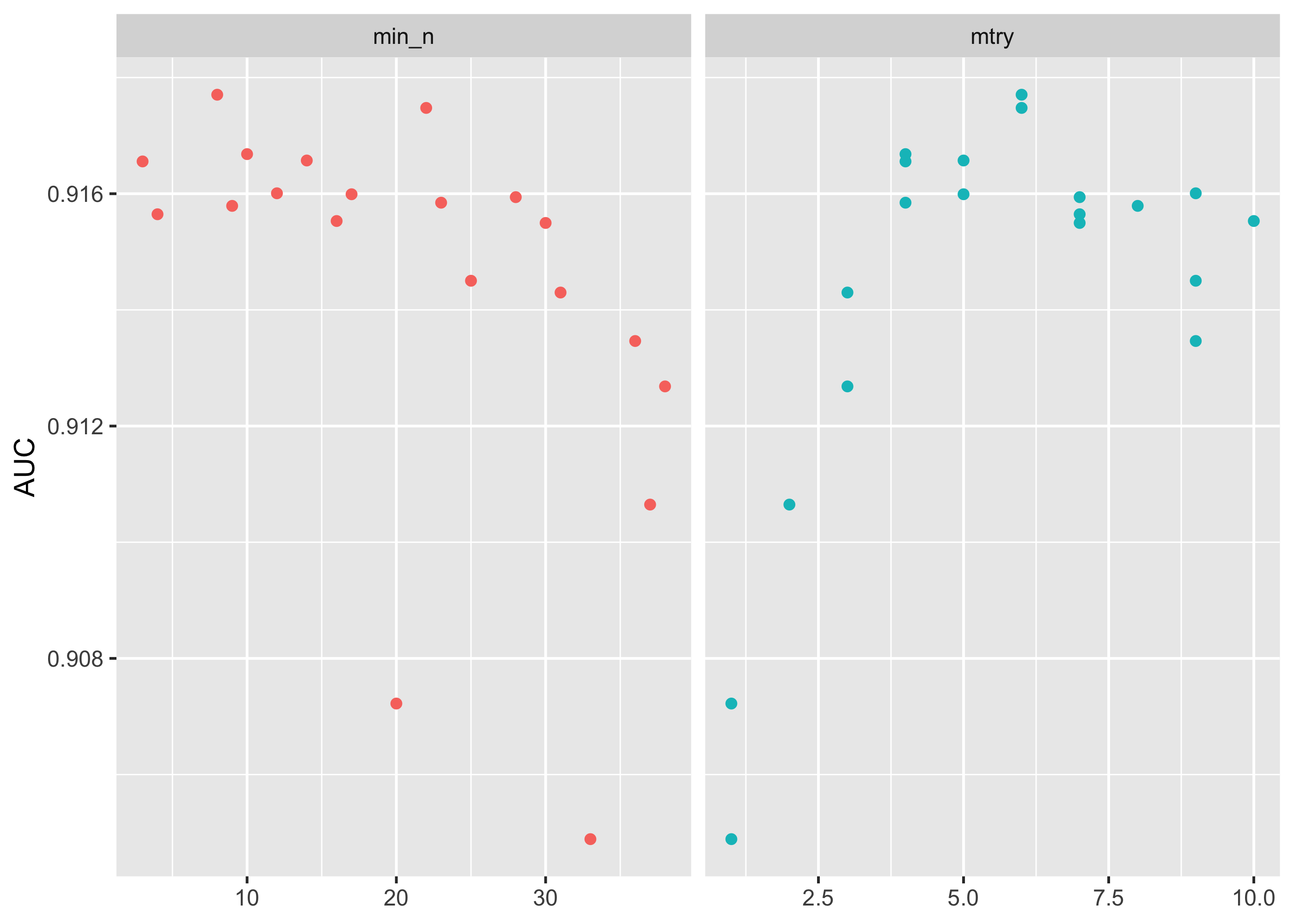
This grid did not involve every combination of min_n and mtry but we can get an idea of what is going on. If we wanted we could test a narrower and more specific range of hyperparameters using the grid_regular() function.
13.3.7 Choosing the best model
Now that we’ve tuned models with several different hyperparameters, we can select the best model with the select_best(), and then update our original model specification to create our final model specification.
best_auc <- select_best(tune_mod, metric = "roc_auc")

final_rf <- finalize_model(tune_spec, best_auc)

final_rf
## Random Forest Model Specification (classification)
##
## Main Arguments:
## mtry = 7
## trees = 1000
## min_n = 12
##
## Computational engine: rangerThis shows that our final model has an mtry value of 6 and a min_n value of 2.
To ultimately see how our good our model is, we want to evaluate predictions from the best model against the test dataset.
To do this, we make a final workflow with our original recipe and our best model final_rf. We can fit it one last time with the function last_fit(), which fits our best model on the entire training set and evaluates on the testing set, when provided with our initial data split.
final_wf <- workflow() %>%
  add_recipe(blgl_rec) %>%
  add_model(final_rf)

final_res <- final_wf %>%
  last_fit(blgl_split)

final_res %>%
  collect_metrics()
## # A tibble: 3 × 4
## .metric .estimator .estimate .config
## <chr> <chr> <dbl> <chr>
## 1 accuracy binary 0.862 Preprocessor1_Model1
## 2 roc_auc binary 0.923 Preprocessor1_Model1
## 3 brier_class binary 0.0934 Preprocessor1_Model1If we collect the metrics from our final model fit we see it has an ROC > .91, where values over .9 are generally considered to be very good.
This suggests that we have a very predictive model for presence of bluegill and one that is not overfit.
Let’s bind our testing results back to the original test set, and make one more map. Where in our pool are there more or fewer incorrectly predicted presences or absences?
# Collect model predictions
preds <- final_res %>% collect_predictions()

# Plot where predictions are correct/incorrect
preds %>%
  mutate(Accuracy = case_when(
    occ == .pred_class ~ "Correct",
    TRUE ~ "Incorrect"
  )) %>%
  bind_cols(blgl_test) %>%
  ggplot(aes(utm_e, utm_n, color = Accuracy)) +
  geom_point(size = 1, alpha = 0.5) +
  scale_color_manual(values = c("gray80", "darkred"))+
  facet_wrap(~paste("Pool",pool), scales = "free")+
  theme_void()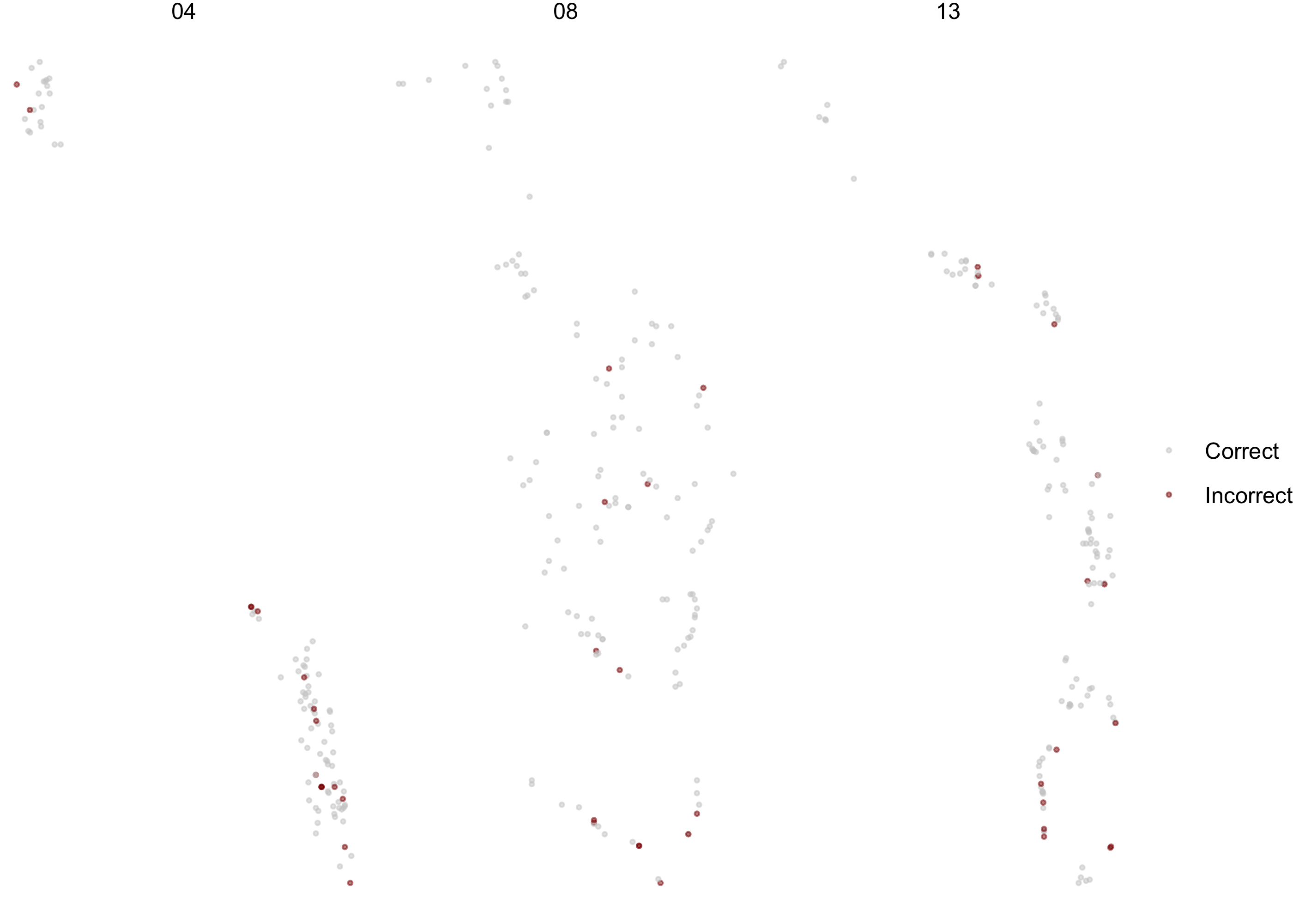
Based on this plot, we may want to dig a bit more into why the model seems to be doing less well in the lower portion of the pools, especially in Pools 4 and 13.
13.3.8 Examine variable importance and partial dependence
We still don’t know what environmental factors matter to bluegill, but there are a couple of ways we can assess this.
First, we can see what variables are most important, using variable importance factors using the vip package.
final_rf %>%
  set_engine("ranger", importance = "permutation") %>%
  fit(occ ~ ., data = juice(blgl_prep)) %>%
  vip(geom = "point")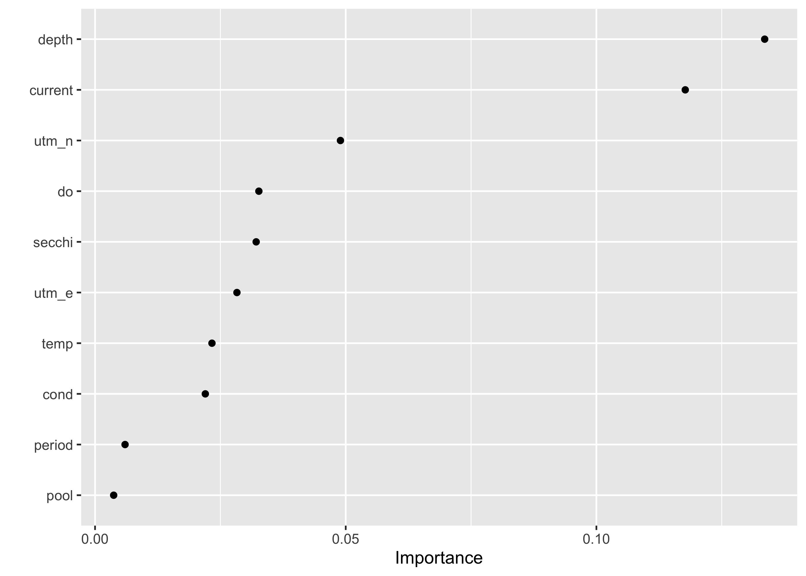
This indicates that depth and current are far and away the most important factors determining the presence of bluegill compared to other factors.
We can also look at how these variables influence the probability of occurrence of bluegill using partial dependence plots, implemented here with the ‘partial’ package.
To make these plots, we first extract the final fitted workflow and model specification (i.e., engine).
final_fitted <- final_res$.workflow[[1]]

rf_engine <- extract_fit_engine(final_fitted)
If we want to predict occurrence of bluegill as a function of depth, we also need to create a new data frame of suitable depth data. Here we pick 50 depth values between 0 and 2.5 meters.
new_depths <- data.frame(depth = seq(0, 2.5, length.out = 50))

head(new_depths)
## depth
## 1 0.00000000
## 2 0.05102041
## 3 0.10204082
## 4 0.15306122
## 5 0.20408163
## 6 0.25510204We can now use the partial package to create our partial dependence data (i.e., predicted occurrence of bluegill as a function of depth). We need to provide our model specification (the rf_engine), what variable we are interested in, the name of the training data, whether we want the output calculated on the probability scale, what class we are predicting (“1” means we are interested in when bluegill are present), and what depths we want to predict for (i.e., new_depths).
pdp_depth <- partial(
  rf_engine,
  pred.var = "depth",
  train = blgl_train,
  prob = TRUE,
  which.class = "1",
  pred.grid = new_depths)
Now we can plot the partial dependence with ggplot. The column yhat represents our predicted probability of occurrence, so that will be on the y-axis.
ggplot(pdp_depth) +
  geom_line(aes(depth, yhat)) +
  labs(
    x = "Depth",
    y = "Predicted occurrence probability",
    title = "Partial dependence plot for bluegill occupancy"
  )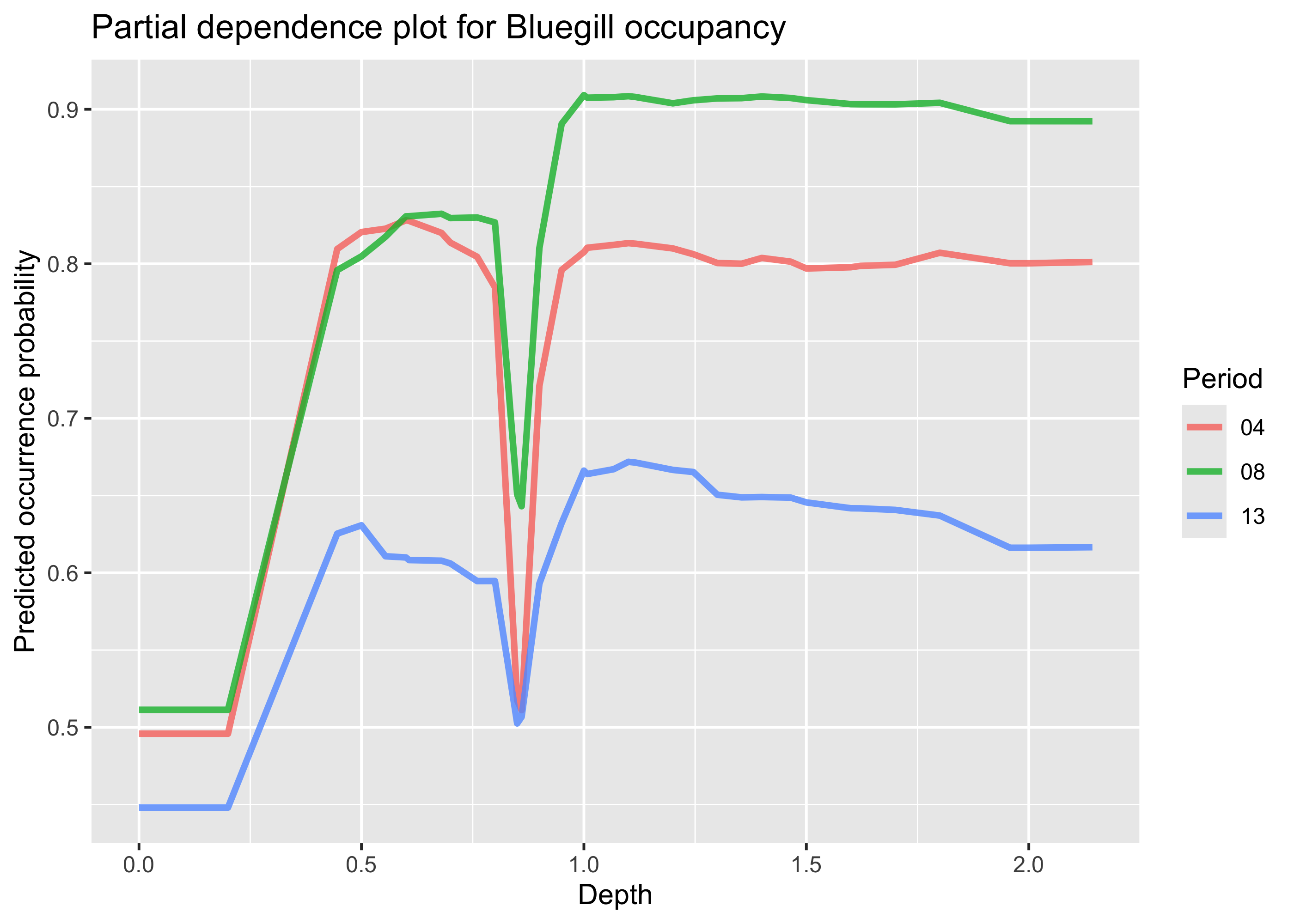
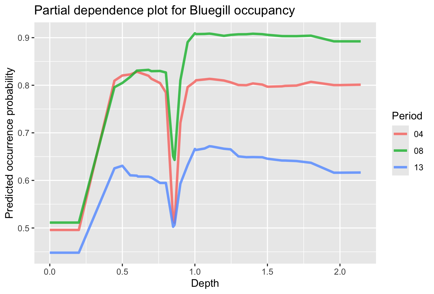
We can see that in general, increases in depths are associated with increased probability of bluegill presence, with maximum occurrence between depths of 0.5 and 0.8 m. The figure shows a sharp dip in probability at depths slightly below 1 m, but this looks likely to be an artifact of the data, and would require more investigation. A plot like this demonstrates the utility of machine learning in planning context. These types of plots can be used to modify existing HSI models that are used for planning, or develop new HSI models. Futhermore, the model itself could be used to predict occurrence of species of interest, and outputs from those models (as opposed to suitability scores) could be used in the planning context once the model is certified.
13.4 Summary
- Machine learning models can excel at prediction if there is adequate data, suggesting it has great potential value for USACE applications
- The
tidymodelspackage provides a complete and comprehensive framework for utilizing numerous machine learning algorithms and carrying out full analyses - Random forest is a powerful, accessible algorithm that can make highly accurate predictions based on tabular data